Tiff maps of predicted Roman marching camp locations
This section lists Tiff maps of predicted Roman marching camp locations across Britain. Maps have been created for various Groups, e.g. Group 65-70 hectares (the Group numbers refer to the size of the camps in hectares). Maps range in size from 1 to 2 megabytes in size. A detailed description of the process to produce these maps is given within this essay. The maps are degraded copies of the originals: if readers require higher resolution versions or detailed maps of an area of interest then please contact the author.
List of marching camp locations at the intersection of rivers and roads, where the river is capable of supplying sufficient water to the marching unit:
List of marching camp locations adjacent to rivers capable of supplying sufficient water to the marching unit:
A generalised legend, showing the colour ranges is available here.
Note:
this essay describes the methods developed to predict the possible
locations of Roman marching camps in Britain. It does not contain,
beyond illustrative examples, any discussion of findings resulting
from this method. For those essays, and information concerning
Boudica's last battle site, the reader is directed to www.bandaarcgeophysics.co.uk/arch_intro.html.
Introduction
This essay describes an attempt to extend the search
for Boudica's last battle beyond the author's earlier work on terrain
analysis work (2010) and hydrology (2012). Essentially this is an
exercise in identifying aspects of the Boudican conflict that might
still be available to modern investigation. Specifically, the camps
built by the Roman force under the command of the Governor, Suetonius
Paulinus, as it retreated from London while being pursued by the
Boudican rebels. As he manoeuvred across southern Britain, his army
would have built and occupied a marching camp each night as part of
the standard operating procedure for Roman units. These camps should,
unless they have been eradicated by the plough or by building, be
still present in the soil profile; but even if not, then a
determination of the possible locations might aid in the tracing of
the legionary footsteps. Such was my reasoning for this exercise. But
what are Roman marching camps?
As mentioned, Roman armies always occupied a
marching camp at night. Either the camp was newly built, or an old
one re-used, often with suitable modification to reflect the new
occupying numbers. The camps may have been occupied for days or weeks
at a time, especially when the Roman army was campaigning, and not at
always by the same unit.
Obviously, these camps were utilised for defensive
purposes, but they also imposed a martial regime and mentality on the
occupiers, thereby magnifying the disciplined nature of the Roman
army. In addition, they were also offensive. Some commentators
suggest that the Romans conquered much of the western world by mobile
trench warfare, whereby the typically smaller Roman forces advanced
into enemy territory camp-by-camp, or trench-by-trench. This was
usually a successful strategy because the tribal opposition was
rarely capable of mounting a siege on a camp and could only hope to
destroy the Roman force during the day and while on-the-move. This is
not to say that Roman camps were never overwhelmed, but this
typically happened after a disaster in battle.
It should be made clear that there are a number of
camp types in the archaeological record: marching, construction,
practice and siege. Differentiating between them is difficult,
sometimes impossible, and in some cases one type would be used for
another purpose, e.g. a former marching camp might become a
construction camp for a local fort. To overcome the inherent
difficulties in deciphering the type and multi-use nature,
archaeologists combine all camp types under the generic term 'Roman
Temporary Camp' (this is not meant to imply a lack of further
classification).
However in this study we are interested in measuring
and classifying some of the physical attributes of camps, that is,
where would Roman surveyors place their camps and why. We are not
concerned with identifying their type. Nor do we wish to
differentiate and classify the camps by period or campaign, for
example, the campaigns of Agricola or Severus in Scotland; that is a
task best left to academic archaeology. For these reasons, this study
makes use of all temporary camps, except those clearly identified as
practice camps, and which have measurable extents, i.e. the length
and breadth are known. Consequently, this study makes use of 374 UK
camps (Figure 1).
The British Isles are blessed with the largest known
number of such camps; typically quoted as greater than 500, but this
number includes re-occupations. Most are located in Scotland, Wales
and the north of England. Unfortunately, probably primarily due to
more aggressive and long-standing agricultural methods, there are
proportionally fewer in southern England, although they almost
certainly did exist in large numbers due to Roman army activity
during the conquest phase and the various tribal revolts.
One purpose of the present study is to try and
identify the possible locations of these missing English camps.
Finally, readers unfamiliar with the story of the
Boudican rebellion, or the author's earlier amalgam of terrain
analysis techniques, known archaeology and the written accounts, are
invited to read www.britarch.ac.uk/ba/ba114/feat3.shtml and www.bandaarcgeophysics.co.uk/arch/boudica-terrain-analysis.pdf . The former is an article published in British Archaeology
(but now without images and maps) and the latter a longer version
with maps. The author's website on the subject is at www.bandaarcgeophysics.co.uk/arch_intro.html (case
sensitive).
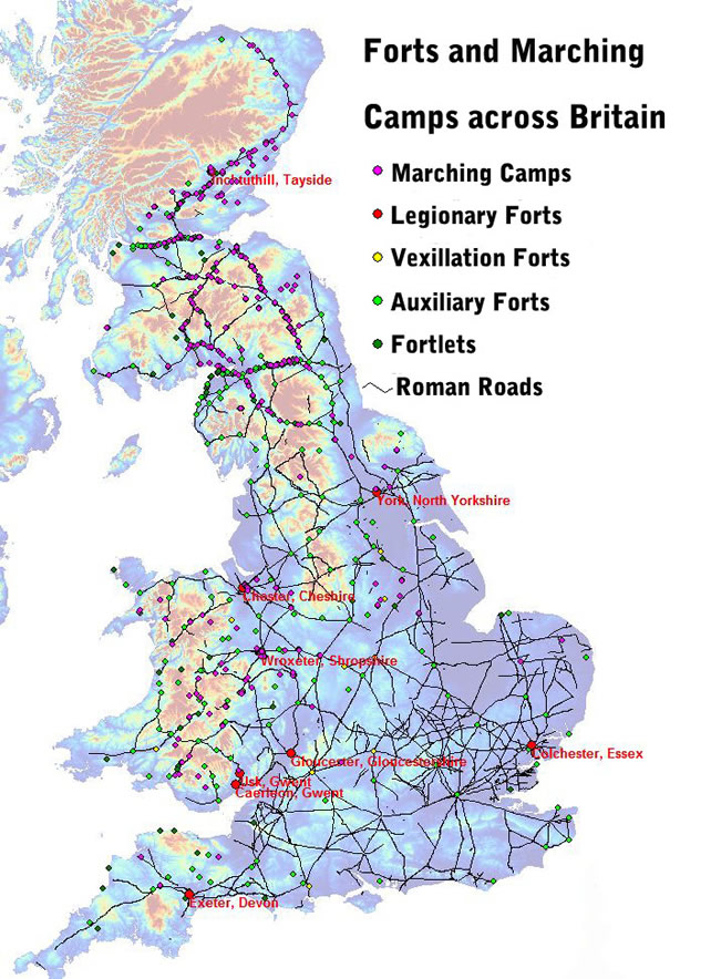
Figure 1:
Distribution of Roman forts, fortlets and marching camps (374) in the
UK. Please note that the depicted Roman roads cover the entire period
of Roman occupation of the islands. Elements of this graph
are © Crown Copyright. All rights reserved 2013.
The Archaeological Data
Figure 1 shows the distribution of known marching
camps used in this study. As already mentioned, there is a lack of
camps in southern England, but this does not mean that they were not
constructed; their surface expression has probably been eradicated by
extensive farming practices and building of many forms. Also, the
apparent lack has largely dampened enthusiasm in the archaeological
community for searching south of the uplands of northern England.
Conversely, greatest number of known marching camps
are located in Scotland and northern England, where there has been a
concerted effort to search for them along routes thought most
favourable. In Wales the density of camps is lower but this may
reflect less interest in finding Roman infrastructure and/or other
archaeological demands. It should be noted that there tends to be a
clustering of marching camps near to Legionary forts, e.g. Chester
and Wroxeter. This may be due to a concentrated effort to study the
surroundings of the fort, and/or Roman army units practising the
building of camps, visiting units setting up camps near to the fort
and the result of punishment details (building a camp is hard work
and would probably have appealed to commanders who had a desire to
discipline the whole unit).
This study includes the camps adjacent to the
Hadrian and Antonine Walls, even though these were probably
construction camps. Nevertheless, they will have been sited in
locations and on ground that will have much in common with those
camps used for campaigning. Removing them from the study would
significantly lower the number used in the study (374) and might
introduce bias in the statistical analysis. The same argument is
applied to construction camps adjacent to fortresses.
The relatively few camps in southern England tend to
be scattered, or randomly distributed, except, as mentioned, for
those adjacent to forts. However, it cannot be denied that during the
conquest period, from 43AD and beyond, the Roman units would have
built and re-used camps; that was their modus operandi.
Whether the camps were still used after pacification is a moot point.
It could be argued that the camps in southern England might have
become sites of mansiones (official stopping or resting places
on roads), then villages and finally, in some cases, towns or cities.
Indeed, there might be merit in extending this present predictive
study of possible marching camps locations to determine if such a
development in useage can be statistically matched to the present-day
sites of villages and towns, i.e. to help answer the question: 'has
much of the building of modern Britain been governed by the location
of Roman infrastructure?' This is an old question, already asked many
times, with the answer repeatedly pointing to the evolutionary nature
of Roman and modern roads and, of course, the towns and cities that
grew around the Roman legionary forts, e.g. York, Exeter and
Gloucester.
Elsewhere, where the marching camps are more clearly
related to operations in hostile territory, the majority of camps
follow route-ways into the land to be conquered or subsequently
controlled. This is most evident in Scotland where strings of
marching camps extend from the south northwards and westwards.
Strings are less evident in Wales, but prime route-ways can still be
discerned.
Figure 1 clearly shows the marked affinity of camps
with Roman roads. Self-evidently the route that the marching legions
would take had been decided upon before the start of the campaign;
camps followed this route and roads, together with forts, fortlets
and towers, were built between the camps. Obviously the marching
camp preceded any other form of infrastructure and, as already noted,
would be re-occupied by units marching up and down the road system.
The initial aim of this study was to acquire more
information that might aid in the hunt for Boudica's last battle,
however, the techniques used and the results gained are thought to be
applicable to many other events in the Roman conquest and occupation
of Britain; future essays will discuss these.
Much could be written in this essay about the known
archaeology but instead the reader is encouraged to make use of the
primary references.
Grouping of the camps
For this study only those camps with known lengths
and breadths were used because a key differentiating attribute is the
area the camp occupied. Of the 374 such camps, Lunanhead in Angus at
86.8 hectares is the largest while Haltwhistle Burn 4 in
Northumberland at 19 x 16 metres, or 0.03 hectares, is the smallest.
However, it may be prudent to consider the possibility that camps
less than 50 x 50 metres might have been practice camps.
Camp size is a characteristic which can be used to
differentiate and group the camps. Please note that the term 'group'
will be used for data arising from this study; this allows a
separation from the term 'series' commonly used by archaeologists for
similar purposes.
The largest camps, i.e. those greater than 30
hectares in size, were not statistically examined, they being few in
number, and grouped as shown in Figures 2, 3 and 4. This resulted in
the groups 65-70 hectares, 50-60 and 40-45. Group 65-70 has a camp
that appears anomalous (Channelkirk, Scottish Borders) caused by a
very low minimum side length (1058 x 512metres and Figure 3) but
nevertheless it belongs within this largest group. The reason for
Channelkirk's anomalous nature is that it sits atop a triangular
shaped peninsular of high ground, bounded by steep slopes on two
sides leading down to rivers, hence the boundary of the camp is
severely constrained by the topography, which forces it away from the
square to semi-rectangular norm of the Roman army.

Figure
2: Graph of groups: plot of the area against the length of the
maximum side Elements of this graph
are © Crown Copyright. All rights reserved 2013.

Figure 3: Graph of groups: plot of the area
against the length of the minimum side. Elements of this graph
are © Crown Copyright. All rights reserved 2013.
An outlier exercise was performed to identify three
camps whose size does not fit within any of the groups in Figure 2.
The largest known camp, Lunanhead in Angus, together with Dunning in
Perth and Kinross, and Raeburnfoot in Dumfries and Galloway are
excluded from the groups, but are included in the exercise to extract
attributes that will be described later.
The first generalised observation is that the Roman
camp surveyors and planners followed a standard rule for specifying
the size of a camp. This rule is almost certainly based on the camp
area required by a specific unit of legionaries, and this is then
scaled to meet the needs of larger groups of men and beasts. Much has
been written about this topic over the centuries of discovery;
details are available in some of the reference material.
The second observation is that the three
largest-by-area groups (65-70, 50-60 and 40-45) are distinctly
separated on the graphs; a fact well-known to archaeologists. Among
the many possibilities for this may be that each group represents the
result of individual campaigns, with each having a different-sized
army or army composition, for example a differing ratio of soldiers
to cavalry.
A third observation is the lack of a group in the
roughly 30 to 40 hectare range, although the range is occupied by the
outlier-camp Raeburnfoot at 32.7 hectares. This may suggest that
groups with areas exceeding 40 hectares were the result of unique
campaigning episodes while the rest of the groups, those less than 30
hectares, represent the normal size of camps used by the Roman army
as it manoeuvred across Britain. This is not to suggest that units
occupying camps less than 30 hectares did not accompany the larger
units, or that the smaller units did not campaign alone.
Figure 4: K-means cluster analysis of camps less
than 30 hectares in size. Note that Cluster 4, with only two camps,
is not designated as a 'group'. Elements of this graph
are © Crown Copyright. All rights reserved 2013.
For camps less than 30 hectares in size the groups
were found by K-means cluster analysis (Figure 4). This exercise
resulted in five clusters based on area, and minimum and maximum
lengths of the side of the camps. Groups 25 hectares, 18, 13, 2.3 and
1.4 were named after the mode of the area in hectares. There is one
outlier cluster (number 4) with just two camps: this has not been
designated as a separate group. The K-means analysis could be allowed
to find more clusters, especially to fill the large apparent gap
between Groups 13 and the next, Group 2.3. This may be beneficial if
the attributes for the camps were extended beyond the area and
perimeter measurements to include others measured in this study; this
may be conducted in the future. Table 1 shows all groups, including
the sub-30 hectare groups.
Group
Name |
Number
of Camps |
Min
Size (hectares) |
Max
Size (hectares) |
Average
Size |
Group
65 - 70 |
3 |
66 |
70 |
67.66 |
Group
50 - 60 |
10 |
51 |
58.6 |
54.68 |
Group
40 - 45 |
7 |
41 |
44.6 |
43.26 |
Group
25 |
25 |
21.2 |
27 |
24.15 |
Group
18 |
48 |
13.7 |
25.5 |
17.21 |
Group
13 |
72 |
6.7 |
13.3 |
10.18 |
Group
2.3 |
88 |
2 |
10.35 |
3.79 |
Group
1.4 |
115 |
0.03 |
4 |
1.03 |
Table 1: some simple area statistics on the
various groups. Elements of this graph
are © Crown Copyright. All rights reserved 2013.

Figure
5: Histogram of groups by number of camps per group and percentage of
group's camps in total number (374). Elements of this graph
are © Crown Copyright. All rights reserved 2013.
Figure 5 re-emphasizes
the unusual nature of the groups larger than 30 hectares; they are
relatively few and, self-evidently, very large. Furthermore in
differentiation, for camps less than 30 hectares there is a linear
relationship between the groups due to the number of camps within
each group, such that Group 1.4 terminates the relationship with the
greatest number. This observation is probably the simple consequence
of far more small units than large ones manoeuvring across Britain,
although it should be remembered that the many of the smaller camps
will have been used for construction at the frontier walls and
fortresses.

Figure
6: Distribution of the largest Roman camps: Groups 65-70, 50-60 and
40-45 hectares. Note that camps of this size are restricted to the
areas shown: there are none in Wales or southern England. Elements of this graph
are © Crown Copyright. All rights reserved 2013.
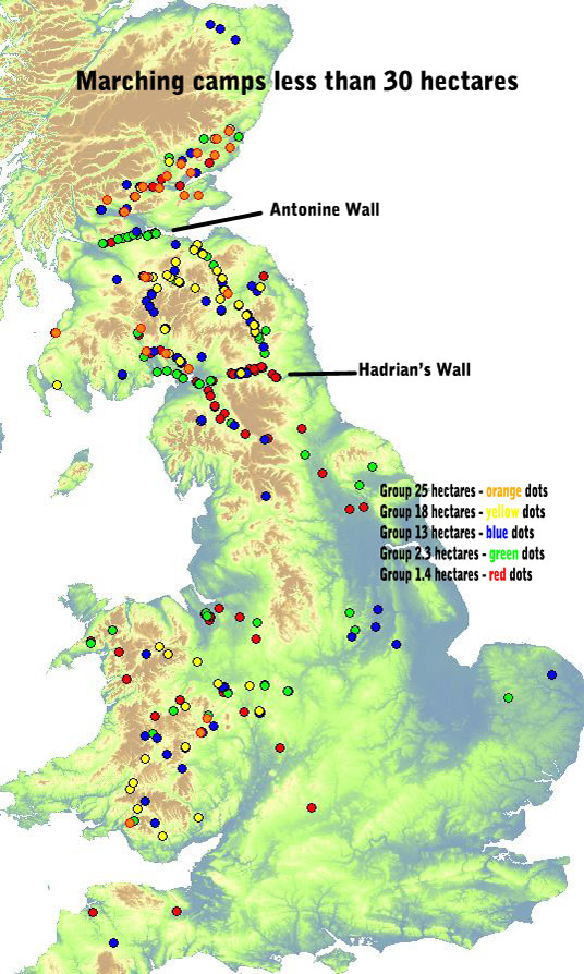
Figure
7: Marching camps less than 30 hectares in size. Groups 25, 18, 13,
2.3 and 1.4 hectares are colour coded. Elements of this graph
are © Crown Copyright. All rights reserved 2013.
Groups
and Series
Archaeologists
of many generations have examined the marching camps in Scotland and
northern England in an attempt to collate them according to size,
number and type of gates, general morphology (e.g. square vs.
rectangular), the commonality of routes and, where appropriate,
dating or assignment to a particular Roman's conquest excursion. The
results are 'series' of camps: the most quoted series are listed in
Tables 2 and 3 (it should be remembered that in this study the camps
are collated into 'groups').
Archaeologist's
Series of Camps |
Groups
of camps from this study |
67
hectares (165 acres) |
Group
65 - 70 hectares |
54
hectares (130 acres) |
Group
50 - 60 hectares |
44
hectares (110 acres) |
Group
40 - 45 hectares |
25
hectares (63 acres) |
Group
25 hectares |
|
Group
18 hectares |
12
hectares (30 acres) – now thought doubtful |
Group
13 hectares |
|
Group
2.3 hectares |
|
Group
1.4 hectares |
Table
2: Comparison of Archaeologist's 'series' and 'groups' from this
study.
There
is some commonality between the series and groups larger than 18
hectares in size, but that hides some differences in detail, for
example, Group 25 includes three camps located in Wales, whereas the
25 hectare series does not cover Wales.
The
creation of groups 18, 13, 2.3 and 1.4 hectares results from
relatively simple statistical analysis and without any attempt to
differentiate on the grounds of location, specific campaign or any
other factor except area and boundary lengths. As such the groups do
appear to cohere because they are necessarily predicated on area
occupied and therefore the relative size of the Roman army units
occupying the camps.

Table
3: Comparison of this study's Groups and archaeologist's Series.
In
keeping with the aim of this essay to describe the predictive method
of finding camps in Britain, the comparison of 'series' and 'groups'
will be curtailed, except to say that in future essays work will be
described that parses the findings in this study relative to the
various series, in an attempt to dovetail the academic archaeological
investigations.
Roman
army units and the numbers of humans in marching camps
In this, and
succeeding sections, the term 'soldier' is used for both a legionary
and auxiliary because in discussing the use of a marching camp, it
cannot be sensibly envisaged that an auxiliary unit was housed (more
accurately, tented), watered, fed and otherwise catered for in a
manner differing greatly from that of a legionary. Additionally,
auxiliary forts are scattered across Britain (Figure 1) which
supposes that there are also an unidentified number of auxiliary
marching camps. In these cases the terms legionary and auxiliary are
interchangeable, hence the preference for 'soldier'.
The area of
each of the 374 selected marching camps can be used to estimate the
numbers of soldiers occupying the camp, that is, the density per
hectare. However, this is not an exact science as there are no
reliable, unambiguous, source statistics. Indeed, this topic has
exercised historians and archaeologists for centuries, and still
does.
Additionally,
the examination of the interiors of UK marching camps has not yet
revealed any firm evidence to support the actual densities of those
camps, or the overall composition of the occupying force.
Luckily for
this study, it appears that a form of consensus has now been reached
in selecting three figures of density of soldiers per hectare that
reflect the likely range the Roman army may have used. These are 480,
690 and 1186 and are based on various studies of known marching or
siege camps, the
historical sources, coupled with knowledge of 18th and 19th century use of army camps.
It is
instructive to observe that the archaeological consensus holds that
the most likely range that reflects the actuality is 480 to 690
soldiers/hectare, and that the 1186 density is simply too compact,
leading to numbers of occupants that seem unlikely - see Figure 8.
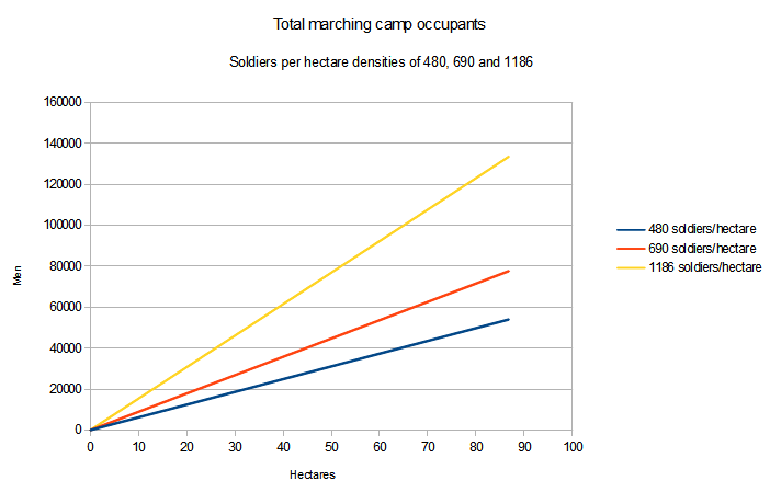
Figure
8: Graph of total number of camp occupants (soldiers and servants)
for 480, 690 and 1186 soldiers per hectare. Note the far steeper
gradient for the 1186 density that results in large, possibly
unreasonable, numbers of occupants. Elements of this graph
are © Crown Copyright. All rights reserved 2013.
For this
study the figure of 690 soldiers/hectare has been selected because
this is the density that seems to most closely approach a realistic figure and is close to those
suggested by the earliest investigators, who were often British army
officers in the 18th and 19th centuries and, therefore, familiar with the camp requirements of
marching troops and cavalry.
The
acceptance of the 690 soldiers/hectare density figure can be
simplified by saying it is the middle-ground – neither too
small (480 men/hectare), nor too large (1186 men/hectare). But a 690
soldier/hectare density is not definitive, objective or necessarily
all-embracing, for undoubtedly there would have been variations
around any density figure depending on the age of camp (1st,
2nd centuries AD etc.), the camp style, the varying topographical
features and, most importantly, the configuration of the army
occupying the camp. For example, an army with an unusually large
cavalry contingent would require a proportionally larger camp than
that occupied by a standard legionary force, hence the density of
soldiers would be lower.
As an aside,
an interesting exercise is to calculate the area available to each
soldier within the camp. At a density of 480 soldiers/hectare each
man had 16.06 square metres: 11.18 m2 at 690 and 6.50 m2 at 1186. These numbers do not take account of the internal layouts
of the camps, the roads or the width of the clear ground
(intervallum)
between the soldiers tents and the camp rampart, because these also
appear to be variable in a number of ways, i.e. there is no
consensus. One might argue that 16.06 m2 is an
overly large space for one soldier, while 6.50 m2 is too small.
As a further
aside, calculating the number of soldiers required to man the
ramparts, at an arbitrary spacing of 1 metre, shows that for the 480
soldiers/hectare density there would have been a reserve force of
approximately 50%: with 60% for the 690 density and 80% for the 1186
density. These figures clearly indicate the strong defensive nature
of the marching camp and supports some of the ancient writers who
report that legionary moral was boosted, when facing the enemy in
open battle, if there was a marching camp to which they could
retreat. These observations re-emphasise the tactical and strategic
importance of the Roman marching camps when relatively small armies
were used to conquer large tribal units. Generally speaking, the
Romans defeated tribal warriors by the use of a disciplined line of
fewer men. To state the obvious, these fewer men could not maintain
that line at night; hence the need of the camp to stop a greater
number of warriors using darkness to overwhelm the Romans. As an
example, the 9th Legion was almost destroyed by a tribal army when campaigning with
Agricola in Scotland; it had encamped and was attacked at night. The
legion was saved by other Roman units rushing to their aid; the
fighting was intense, both within the camp and at the gates. In all
probability the 9th would have been destroyed without the defensive capacity of its
marching camp. Supporting this line of reasoning are the accounts of
Roman army units being collectively punished by being made to pitch
their tents outside of the camps, an act obviously seen as dangerous.
To return to
the primary theme of this section, given the area of each camp and
the preferred density of 690 soldiers/hectare, we can estimate the
numbers of soldiers, servants and slaves, mules and horses in
occupation. These estimates are based on generally accepted standard
numbers for Legionary forces, specifically the legionary cohort
system of the early Roman Empire of the 1st and 2nd centuries AD. This study does not attempt to vary these legionary
numbers due to the presence of auxiliary, siege equipment or
additional cavalry units, beyond those cavalry normally assigned to a
legion. To attempt to do otherwise would require an extremely complex
investigation of each individual camp and, by necessity, lead to a
detailed analysis of the historical reasoning for the existence of
the camp. In emphasis therefore, the number of soldiers etc. in each
camp is anchored on the generally accepted legionary standard of:
a
basic unit of 8 soldiers contubernium),
a centuria consisting of 10 contubernium = 80 soldiers,
a standard cohors consisting of 6 centuria = 480 soldiers,
a legion consisting of 9 cohors> of 480 soldiers and one 1st cohors of 800 soldiers = 5120 soldiers.
Each contubernium was supported by at least two servants and the same number of mules
used as baggage transport. Typically 120 cavalry are attributed to a
legion, but in this study this is doubled to reflect the probable
presence of at least one remount; there may have been more. The
resulting figures for a standard legion of 5120 soldiers and for St.
Leonard's Hill, the largest known camp, are in Table 4. It should be
stated that these numbers exclude officers, their servants and
supernumeraries.
Camp |
Area
(hectares) |
Soldiers |
Servants |
Mules |
Cavalry |
Total
humans |
Standard
Legion |
7.42 |
5120 |
1280 |
1280 |
240 |
6520 |
St.
Leonard's Hill |
70 |
48300 |
12075 |
12075 |
2264 |
61507
|
Table 4:
Numbers of soldiers, servants, mules and cavalry for two camps based
on a density of 690 soldiers/hectare. St. Leonard's Hill is the
largest known camp in Britain. Lunanhead at 86 hectares is the
largest but is thought to be atypical in its use, the boundaries are
not confirmed and it is classified as a 'probable' camp by
archaeologists. Elements of this graph
are © Crown Copyright. All rights reserved 2013.
The
reader is invited to compare the numbers in Table 4, at a density of
690 soldiers/hectare, with those in Table 5 at densities of 480 and
1186 soldiers/hectare (the area is fixed between the tables).
Camp |
Area(hectares) |
Soldiers |
Servants |
Mules |
Cavalry |
Total
humans |
Standard
Legion at 480 |
7.42 |
3561 |
890 |
890 |
166 |
4534 |
Standard
Legion at 1186 |
7.42 |
8800 |
2200 |
2200 |
412 |
11206 |
|
|
|
|
|
|
|
St.
Leonard's Hill at 480 |
70 |
33600 |
8400 |
8400 |
1575 |
42787 |
St.
Leonard's Hill at 1186 |
70 |
83020 |
20755 |
20755 |
3891 |
105720 |
Table 5:
Same calculations as for Table 4 but for camp densities of 480 and
1186 soldiers/hectare. Elements of this graph
are © Crown Copyright. All rights reserved 2013.
Probably
the most striking feature of the comparison is the size of the
numbers for St. Leonard's Hill at a density of 1186 soldiers/hectare,
i.e. 83,020 soldiers, 20,755 servants and 1,945 cavalrymen, giving a
total of 105,720 humans. That number of soldiers equates to
approximately 16 full legions (at 5200 legionaries per legion); an
extremely large legionary force if taken at face value. However, it
has been estimated that six legions (that is c.30,000 legionaries)
were campaigning under the Emperor Severus when the camp at St.
Leonard's Hill was built. If, as seems to have been normal Roman
practice, each army consisted of an equal number of legionaries and
auxiliaries, i.e. 60,000 soldiers, then the 83,020 figure appears a little more credible but, a difference of c.20,000 soldiers is still a large
discrepancy and adds weight to the earlier description of the
consensus suggesting the density of 1186 is too large.
In
comparison, examining St. Leonard's Hill at a density of 480
soldiers/hectare, and assuming that the previously mentioned estimate
of c.30,000 legionaries is correct, suggests that the calculated
number of soldiers at 33,600 is too low for that campaign, there
being an insufficient number of auxiliaries to match the normal Roman
practice. Unfortunately the same argument, but to a lesser extent,
can be made against the calculation density used in this study of 690
soldiers/hectare. Such is the difficulty of selecting the most
appropriate density for the camps in Britain.
Statistical
analysis of camps
Having
calculated the areal size, numbers of humans, mules and horses for
all 374 known marching camps we can now make use of modern
topographical datasets to assist in identifying those features and
parameters that the Roman camp surveyors thought suitable when
choosing a camp site. In this manner we can try to understand what a
surveyor was thinking of and what rules he was operating under as he
examined the terrain his commander had chosen to advance over.
The
primary topographic dataset is the Shuttle Radar Topography Mission
(SRTM) with a grid spacing of 90 metres (see the background in Figure
1). Other publicly available datasets at 50 metre spacing were
examined but these contained too much detail from the modern era
(cities, towns, roads, rail, river alterations, field and drainage
lineaments, etc.) which caused a wide range of errors in the
processing conducted for this study. Conversely, the SRTM 90 metre
spacing produces a relatively smooth topographic surface, largely
removed of modern artefacts and can be classed as artificially
naturalised, i.e. a gridded surface of topography lacking most of the
human additions of the last 2000 years. Nevertheless, a higher
definition dataset, devoid of modern attributes, would produce a set
of results of finer detail. This observation pertains to all the work
presented in this study.
Prior
to all computations the SRTM 90 metre spacing was up-scaled to 50
metres which allows for higher
definition in the measurements of distances associated with allied
datasets, e.g. the precision in locations of the known marching
camps. The primary software used in this study, SAGA (see references), was used to produce from the SRTM data the following grids of
simple attributes for Britain:
- Curvature
(tangential) of the topography - curvature
in an inclined plane perpendicular
to the surface – a measure of flatness,
- Openness
of the topography – how much the camp would have been
over-looked, e.g. a hill over-looking a plain – a measure of
camp safety,
- Ruggedness
– the average
elevation change between any point on a grid and its surrounding
area – a measure of ground undulation or roughness,
- The
SAGA Wetness Index – calculation of soil moisture or
saturation – a measure of water-logging,
- Slope
– the standard slope of a surface – a measure of camp
drainage,
- Topographic
Position Index (TPI) - the
difference between a cell elevation value and the average elevation
of surrounding cells – a measure of the type of ground,
- TPI
land form – a classification derived from 6, the TPI – a
measure of the type of topography,
- Distance
to Roman roads - a measure of suitability for advancing a campaign,
or differentiation between standard manoeuvring and advancing to
contact/battle.
Figure
9 is a montage of some of these attributes for the Kennet river
catchment in Berkshire.
There
are a large number of topographic indices and descriptors that could
have been calculated, but those above were chosen for their
simplicity and direct relationship to the likely thought processes of
the Roman surveyor. Other indices may be calculated in the future if
it is thought they provide further insights. Clearly missing in the
list is any reference to rivers which will be dealt with in the next
section.

Figure
9: montage of computed topographic attributes for an area with in the
Kennet river catchment. The attribute type, clockwise from top left,
is curvature, SAGA wetness, topographic position index (TPI), TPI
land forms, ruggedness and openness.
Water:
calculation of supply and demand
What
follows is a précis of the author's primary work on the water
needs of the Roman army and the available water supply in Britain –
the demand and supply. The full description of the work conducted on
this subject can be found in:
Boudica-logistics.pdf
( www.bandaarcgeophysics.co.uk/arch/boudica_logistics.pdf ) and
the author's website at www.bandaarcgeophysics.co.uk/arch_intro.html .
The
primary work concluded that the average soldier needed to drink at
least 9 litres of water per day. This figure is for a marching,
rampart and ditch digging, foraging and fodder collecting individual,
weighted down by 43 kilograms of clothing and equipment, and
operating at a temperature of 20-25oC in a temperate climate, i.e. a typical August day in Britain. The 9
litre/day figure does not include that required for cooking, washing
etc..
Water
requirement figures were estimated for hard-working mules and horses
at 30 and 70 litres per day, respectively. Table 6 displays the water
requirements for a Roman army of 10,000 soldiers plus supporting
staff and beasts. Table 7 provides the total for the army from the
values in Table 6, and displays the results in cubic metre per second
(cumec) corrected for the available daylight in August (the
assumption is that night-time collecting of water from rivers would
not be allowed – too dangerous). The final figure of 0.00386
cumec was the minimum that the rivers adjacent to the camp would need
to supply to match the demand.
|
Soldiers |
Servants |
Horses |
Mules |
Number
of |
10000 |
2500 |
468 |
2500 |
Water
required (litre/day) |
9 |
9 |
70 |
30 |
Sum
(litre/day) |
90000 |
22500 |
32812 |
7500 |
Table 6: The water requirements of 10,000
soldiers, servants, horses and mules.
|
Litres |
Cubic
metres |
Cubic
metres/second |
Cubic
metres/second - daylight corrected |
Total
Army water requirement |
220312 |
220.31 |
0.00255 |
0.00386 |
Table 7:
Total army water requirement: sums from Table 6 converted to cubic
metre/second (cumec) and corrected for the available daylight in
August.
The
same calculations were conducted for all 374 known marching camps.
The
next stage was to calculate the hydrology for the whole of Britain
(Figure 10) which would ultimately indicate where the camps could
have been sited alongside rivers with flow sufficient to satisfy the
camp demand. Conversely, and equally importantly, the measurement of
the river flows in August, the selected month based on the most
probable high point of the campaigning season, indicates where
marching camps of specific size would not be sited. This is not to suggest that marching camps were never
placed in locations without sufficient water, but that would probably
have been a choice borne of operational necessity, for example,
occupying a hill-top in preparation for a localised skirmish or
battle the following day. What is undoubtedly true, and for obvious
reasons, is that army commanders do not habitually place their units
in locations where there is a lack of water: to do otherwise is to
court disaster.
The
minimum calculation of river flows was limited to 0.0003 cumec
because of the inherent inaccuracy of the calculation method at such
low rates. Consequently, only those marching camps with a total water
requirement exceeding 0.0003 cumec (307), continued in the study.
Those removed have areas less than 1.15 hectares and contained less
than 793 soldiers – approximately two cohorts at a density of
690/soldiers/hectare.

Figure
10: The computed, naturalised hydrology of Britain. Main image shows
all rivers that have a flow greater than 0.05 cumec in August. The
inset shows all rivulets, streams, and rivers for the Kennet river
catchment in August.
Calculation
of topographical and hydrological attributes for known marching
camps.
Having
calculated the grids for topographic attributes, e.g. curvature and
slope, and the same for hydrology, e.g. river flow rates, the next
stage was to use the locations and known boundaries of the remaining
307 marching camps to extract those attributes that pertained to each
camp, and calculate suitable statistics from them. This was a
relatively simple exercise, but one cluttered with computational and
statistical detail which, it is felt, most readers would probably
find tedious to read: for that reason we shall only examine a few key
illustrative points.
As
a reminder, this exercise was designed to discover some of the
factors that a Roman army surveyor might have thought important when
choosing the location of a marching camp.
Some
attributes are important only within the camp ramparts; others
maintain their importance some distance beyond. An example of the
former is the ruggedness of the topography, which was used as a proxy
for the amount of level ground within the camp suitable for the
setting of tents. For the latter, the attribute of openness was
determined for a set distance (buffer) around the camp. The openness
is a measure of the tactical suitability of the camp, in the sense
that a camp ground closely overlooked by a hill would offer an enemy
the ability to spy and launch missiles. Therefore, a camp itself
located on a hill and surrounded by lower elevation plains or
valleys, is very open, i.e. very suitable for the Romans; conversely,
a camp sited within, say, Cheddar Gorge would have a very low
openness for obvious reasons, i.e. it is very unsuitable.
An
obvious set of attributes that nearly always required the examination
of features external to the camp ramparts were those of hydrology;
rarely do camps have substantial streams running through them.
However, some do contain rivulets with flow rates less than the
study's lower limit of 0.0003 cumec. The grid of river flow rates for
the whole of Britain was examined around each of the 307 known camps
at 50, 100, 200, 300, 400, 500, 750, 1000, 1500, 2000 and 3000 metre
distances. Three kilometres might be considered an excessive distance
from the camp, but it was chosen to include the possibility that
patrolling cavalry might have used rivers at that distance to water
their mounts. The added benefit is that some of the rivers at one,
two and three kilometres are very large and hence form a barrier to
enemy advancement. This factor has not been examined in this study as
it is very specific to each camp, but may be in the future.
The
total number of topographical and hydrological attributes is listed
in Table 8. For the topographical attributes the value of each grid
cell was found and the average, mode, median, maximum, minimum and
standard deviation were calculated for the 307 camps. A similar
exercise was performed on the hydrology cells but statistics were
also calculated for both the river flow rate and the distance from
the camp rampart to the river(s).
Attribute
Type |
Attribute |
Topographical |
Curvature |
|
Openness |
|
Ruggedness |
|
Wetness |
|
Slope |
|
Topographic
Position Index (TPI) |
|
TPI
land forms |
|
Distance
to Roman roads |
|
|
Hydrological |
Height
of camp above river |
|
River
flow rates at 50, 100, 200, 300, 400, 500, 750, 1000, 1500, 2000
and 3000 metres |
|
Distances
to first, second, third and fourth rivers |
|
Flow
rates of first, second, third and fourth rivers |
|
Distance
to the first river that supplies sufficient water to the camp |
|
Distance
to the second river (and so on) that supplies sufficient water to
the camp |
Table 8:
Attributes extracted and computed from the topographical and
hydrological grids.
Distances
of rivers from the marching camps
The
examination of the hydrology surrounding the 307 marching camps
allows insights into the use of rivers and streams by the Roman army
surveyors. The large statistical dataset described in the preceding
section can be further computed, resulting in some interesting
observations. However, it should be remembered that the base
topographical data (SRTM) is at 90 metre resolution which implies
that the accuracy of distance measurements of a river to a camp is in
the range of 45 metres, whereas, the reality was that rivers may have
been closer, in some cases, than that reported in this study; some
were also further away. However, because the SRTM data has been made
hydrologically sound and naturalised, the reported distances to
rivers and streams is in many cases superior to those that would be
computed from high resolution, modern maps. This is especially true
for smaller streams and rivers which, over the 2000 year history of
agricultural improvement, particularly the use of drainage schemes,
have either been removed or greatly altered. Nevertheless, a higher
density, hydrologically sound and naturalised topographical dataset
would produce higher fidelity results, that is, closer to the
actuality seen by the Roman army surveyor.
The
first set of observations relate to the general distribution of
rivers and streams around marching camps. Table 9 and Figure 11
display the distance statistics for the closest river to a camp. Of
the 307 camps, 139 (45.27%) have rivers within 50 metres of the
rampart. A further 44 camps have rivers within 100 metres, giving a
cumulative frequency of 59.61%. Continuing, we can see that almost
90% of camps have rivers within 300 metres. It might appear
surprising that 10 camps have rivers further away than 750 metres
but, I tentatively suggest, these camps may have a location more
tuned to a local tactical need, e.g. occupying a hilltop to deny the
enemy. Observations of this nature will be tested in work yet to be
conducted.
If
59.61% of all the camps were placed within 100 metres of rivers, then
the general observation that water supply was a critical
consideration when placing the camps can be supported with
confidence. Of course, water supply is not all that rivers provide.
They also have defensive benefits and these can be compounded by a
second local river, Table 10 and Figure 12.
Distance
to 1st river |
Frequency |
Relative
frequency |
Cumulative
frequency |
50 |
139 |
45.27 |
|
100 |
44 |
14.33 |
59.61 |
200 |
59 |
19.22 |
78.83 |
300 |
34 |
11.07 |
89.9 |
400 |
14 |
4.56 |
94.46 |
500 |
7 |
2.28 |
96.74 |
750 |
9 |
2.93 |
99.67 |
1000 |
1 |
0.3 |
100 |
1500 |
|
|
|
2000 |
|
|
|
3000 |
|
|
|
Table 9:
Statistics on the distances to the 1st river.
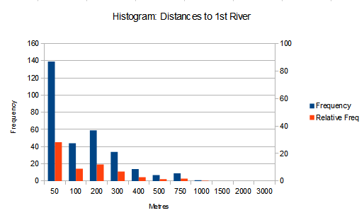
Figure
11: Histogram of distances to the 1st river closest to marching camps.
Distance
to 2nd river |
Frequency |
Relative
frequency |
Cumulative
frequency |
50 |
0 |
0 |
|
100 |
45 |
17.05 |
17.05 |
200 |
66 |
25 |
42.05 |
300 |
42 |
15.9 |
57.95 |
400 |
39 |
14.77 |
72.72 |
500 |
17 |
6.44 |
79.16 |
750 |
22 |
8.33 |
87.5 |
1000 |
16 |
6.06 |
93.56 |
1500 |
7 |
2.65 |
96.21 |
2000 |
8 |
3.03 |
99.24 |
3000 |
2 |
0.75 |
100 |
Table 10:
Statistics on the distances to the 2nd river.

Figure
12: Histogram of distances to the 2nd river closest to marching camps.
Of
the 307 camps under examination, 264 had a second river within the
3000 metre examination range. Given that range, and a wet country
such as Britain, this is not surprising. More significantly, Table 10
shows that 42% and 72% of camps had 2nd rivers within 200 and 400 metres, respectively. Individual camps have
not yet been visually examined, so no comment can be made regarding
the flow relationship of the 1st and 2nd rivers, for example, if one is a tributary of another or they are two
separate rivers. In either case, it seems probable that the camp
surveyors were deliberately choosing sites bounded by at least two
river courses and, in some cases, placing the camps close to the
junctions of tributaries. The defensive qualities of such
arrangements are obvious.
Please
note that these apparently large distances to rivers might seem too
far away from a camp but, of the 307 camps under study, 103 have
boundaries in excess of 400 metres on at least two sides. Therefore,
the scale of the camps and the number of men and beasts they
contained, was large, thus requiring a similar scale for the supplied
resources (water, pasture, forage and fodder) and the defensive
qualities of the surrounding land and rivers. Additionally, the
nature of Roman legionary warfare, when faced with tribal enemies,
suggests that the daylight hours were relatively safe for the Romans.
Under normal circumstances they could control the resource hinterland
by the use of foot and cavalry patrols, such that they would have
warning of an approaching enemy and be able to retreat to the camp,
or form-up into a battle array. At night the hinterland was probably
vacated by the Romans – hence the punishment of making units
site their tents outside of the ramparts – and reclaimed each
morning.
We
can conclude the discussion of distances by noting that 205 camps
have at least three close rivers and that 51% of those have a third
river within 500 metres, Table 11 and Figure 13.
Distance
to 3rd river |
Frequency |
Relative
frequency |
Cumulative
frequency |
50 |
0 |
0 |
0 |
100 |
0 |
0 |
0 |
200 |
16 |
7.8 |
7.8 |
300 |
31 |
15.12 |
22.93 |
400 |
26 |
12.68 |
35.6 |
500 |
32 |
15.61 |
51.22 |
750 |
33 |
16.09 |
67.32 |
1000 |
15 |
7.32 |
74.63 |
1500 |
24 |
11.7 |
86.34 |
2000 |
13 |
6.34 |
92.68 |
3000 |
15 |
7.32 |
100 |
Table 11:
Statistics on the distances to the 3rd river for 205 of 307 camps.
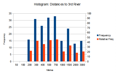
Figure
13: Histogram of distances to the 3rd river closest to 205 of 307 marching camps.
As
already mentioned, the placing of marching camps close to multiple
rivers and/or their junctions confers an obvious defensive benefit to
the Romans. However, there may be other benefits, namely, the use of
different rivers for different purposes.
Ancient
writers and military officers of the 19th century describe, in general terms, the management of water resources
by large bodies of soldiers and beasts. It is advised that the
soldiers should extract water for drinking and cooking purposes from
the upper reaches of the river. Further downstream the soldiers
should use the river for bathing and laundry washing. Lower reaches
of the river course are the preserve of the horses and, in the case
of a Roman army, the mules. If cattle are being driven with the army,
then they should make use of the lowest reach, as they are prone to
destroying river banks and muddying and fouling the river. In many
accounts it is noted that horses can be difficult, even fussy, about
the quality of their drinking water and may require preferential
drinking arrangements; mules, being generally more robust, will drink
from contaminated water and should be watered below the horses.
Therefore
the following string indicates the order of water use ( >
represents further downstream) :
soldiers
drinking and cooking > soldiers bathing and laundering > horse
> mules > cattle.
The
availability of multiple rivers adjacent to camps offers the
possibility of separating the soldiers' use of rivers from that of
the beasts, i.e. one river for soldiers, another for horses and
possibly another for mules and cattle. This, or similar arrangements,
clearly confers benefits to all occupants of the marching camp, but
especially the soldiers. Variations of the general scheme can be
envisaged; for example, in large camps with many thousands of
soldiers, they may have used two rivers while the beasts used
another, probably the most distant river they encountered as they
were led to grazing.
There
is another use of rivers by soldiers that may have occurred - to
flush latrines. It is well documented that the Romans used water
flows to flush their communal latrines in forts, towns and cities.
Although no evidence has yet been found for such use in marching
camps, surely it would not be surprising if such were found.
It
is worthwhile examining the effluent problem in some detail. A study
of civilians in the 1960s produced the first recorded figures on the
quantity of human effluent. Unfortunately, the author is not aware of
a similar study for active soldiers who require considerably more
energy and hydration, with concomitant effluent output, than the
average civilian. Nevertheless, we can use the civilian figures to
gauge the effluent problem relating to a large marching camp, but
also remembering that the figures are considerably underestimated.
Hence the study showed that civilian men produce an average of 0.498
kg of solids per day.
Using
these figures and applying them to the Newsteads V marching camp
(approx. 60k humans at a density of 690/hectare) gives a figure of
37.87 metric tonnes of solids each day which is 265 tonnes a week. As
a means of putting these numbers in perspective, this is the weight
of 18 London double-decker buses. By volume the solids occupy 37.97
cubic metres each day (Figure 14) and 265 a week.

Figure
14: This trailer has a rated volume of 38 cubic metres, i.e. the same
volume of solids produced by 60,000 humans at Newsteads V each
day.
Clearly,
managing the amount of solids produced was a considerable problem,
especially so when the marching camps might have been occupied for
days or weeks at a time, and re-occupied by varying force-sizes
during and after that year's campaigning. We can examine the
management issue by relating these production figures to studies
conducted by the US Army.
The
US army has conducted measurements of the use of a standard
'straddle-trench' latrine, where after use the soldier covers and
in-fills the deposit with soil. If the fill ratio of the trench is
75% soil and 25% human solids, then Newsteads V would have needed 548
trenches each day, covering an area of 601 square metres. For a week,
this is 3836 trenches covering 4207 square metres or 0.4207 hectares.
To-date
none of the pits etc. located within the ramparts excavated in
Britain has shown evidence of latrine use. However this does not mean
that they did not exist as the remains may have been destroyed over
time. Nevertheless the size of the management issue suggests that the
latrines were probably
located outside the camp but close enough to be readily guarded
during the day by patrolling foot and cavalry. Of course, there would
have been a need for some latrines within the camp to accommodate any
night-time needs.
The
amount of continuous effort needed to dig and maintain the large
number of latrines, the local proximity by choice of numerous rivers
and streams, and the known expertise with which the Romans elsewhere
managed effluent by water flow, suggests the possibility that the
rivers and streams near camps may have been similarly utilised. Might
the camp occupants have simply dug a trench sub-parallel to a river
or stream then connected it at either end to allow water to flow
through? Simple, effective and well within the engineering capacity
and capability of the Romans. And of course, choosing a single river
for waste disposal, while using others for water extraction and
drinking, literally carries away the possibility of noisome fouling
of the camp and grounds, and diminishes the possibility of disease
transmission.
It
should be made quite clear that there is no evidence, written or
otherwise, to confirm this hypothesis but, given the Roman
predilection for soldierly-cleanliness and their keenness for
engineered solutions, it seems to this author to have merit.
Water:
the matching of demand and supply
In
this section we shall examine the water requirements of all of the
humans and beasts occupying the camps and the water available from
rivers and streams, i.e. the demand and supply.
Having
used a density of 690 soldiers/hectare, assessed the number of beasts
present by commonly accepted ratios, and knowing the water needs of
each, we can calculate the total water requirement for each of the
307 measured marching camps (example in Tables 6 and 7), that is, the
demand.
The
supply side was calculated individually for each river and stream
adjacent to the camps out to a distance of 3km. Knowing the distances
to, and the supply from, each river allowed the calculation of
cumulative supply rates. From these relatively simple statistics some
interesting observations can be made.
Of
the 307 camps, 23.78% receive their total demand within 50 metres of
the ramparts: 37.46% within 100 metres, 63.84 within 200 metres and
78.16% within 300 metres ( Table 12 and Figure 15).
Distance
to river(s) |
Frequency |
Relative
frequency |
Cumulative
frequency |
50 |
73 |
23.78 |
0 |
100 |
42 |
13.68 |
37.46 |
200 |
81 |
26.38 |
63.84 |
300 |
44 |
14.33 |
78.16 |
400 |
30 |
9.77 |
87.94 |
500 |
16 |
5.21 |
93.16 |
750 |
13 |
4.23 |
97.39 |
1000 |
6 |
1.95 |
99.35 |
1500 |
2 |
0.65 |
100 |
2000 |
|
|
|
3000 |
|
|
|
Table 12:
Statistics on the distances to the river(s) that totally supply the
camp demand.

Figure
15: Histogram of distances to the river(s) that totally supply the
camp demand.
These
statistics again support the observation that the Roman surveyors
were placing their camps close to rivers and streams, and that they
probably had some method of estimating the supply capacity of the
local water sources and matching this to the demand. One might be
tempted to think that the statistics simply indicate the obvious,
that of course the Romans placed their camps next to rivers that
would supply enough water. However, the surveyors selection of sites
appears to have been more complicated than that. For example, if
water supply was the prime consideration then one might expect the
camps to have been placed alongside a river that totally supplied the
demand, but Table 12 and Figure 15 shows this was not the case. Other
factors were certainly being taken into account, such as the need to
use the rivers and streams for defence, the need to distribute the
water supply for soldiers and beasts along different water courses,
and the acceptance that during the night the camp hinterland and
rivers would be no-go areas but reclaimed each morning as the patrols
pushed outwards the area of direct Roman control. In other words, the
overall defence of the camp may have been deemed more important than
the easy, close access to sufficient water. However, it should be
remembered that the construction camps for the Antonine and Hadrian
walls that are included in this study were probably located primarily
for their purpose. For the rest, no doubt other factors in location
played an important role, as we shall investigate.
The
balance between water supply and other factors is further emphasised
by examining the frequency of the closest and second-closest rivers
in supplying the total demand (Tables 13 and 14, respectively). Of
the 307 camps under examination, there are 194 closest rivers which
satisfy the demand of which: 24.1% of the 307 are within 50 metres;
34.2% within 100 metres; and 56.03% within 300 metres. Similarly,
there are 72 camps of the 307 which, when the supply from the closest
and second-closest rivers are combined, supply the totality of
demand, such that: 3.58% are within 100 metres; 13.68% within 200
metres; and 18.57% within 300 metres.
Distance
to river |
Frequency |
Pop.
Relative frequency |
Pop.
Cumulative frequency |
50 |
74 |
24.1 |
|
100 |
31 |
10.09 |
34.2 |
200 |
44 |
14.33 |
48.53 |
300 |
23 |
7.49 |
56.03 |
400 |
11 |
3.58 |
59.6 |
500 |
5 |
1.62 |
61.23 |
750 |
8 |
2.6 |
63.83 |
1000 |
1 |
0.33 |
64.17 |
1500 |
|
|
|
2000 |
|
|
|
3000 |
|
|
|
Table 13:
Frequency statistics on the closest river that totally supplied the
camp demand.
Distance
to river |
Frequency |
Pop.
Relative frequency |
Pop.
Cumulative frequency |
50 |
|
|
|
100 |
11 |
3.58 |
|
200 |
31 |
10.1 |
13.68 |
300 |
15 |
4.89 |
18.57 |
400 |
11 |
3.58 |
22.15 |
500 |
2 |
0.65 |
22.8 |
750 |
1 |
0.33 |
23.13 |
1000 |
3 |
0.98 |
24.1 |
1500 |
|
|
|
2000 |
|
|
|
3000 |
|
|
|
Table 14:
Frequency statistics on the closest and second-closest rivers that,
in combination, totally supplied the camp demand.
Further
examination shows that the closest and second-closest rivers, that
either singularly or in combination provide enough water to match the
demand, account for 271 of the 307 camps, i.e. 88.27%. Necessarily
therefore, 36 camps (11.73%) require the water supply from a third
river (31 camps or 10.09%) and a fourth (5 camps or 1.63%) to match
the full demand of those camps (Note: a maximum of only four rivers
per camp were differentiated in this study; there may be more). The
31 camps that required the use of a third river, all of which lie
with the range 200 to 1500 metres from the camp ramparts, suggests
that these may have been more sensibly used to water the beasts. This
may also be true of the fourth rivers but, at only 1.63% of the total
camp population, the water demand and supply calculations border on
the unsupportable.
In
the quest to discover what it was that the Roman surveyor was
thinking of when examining a landscape and rivers, use can be made of
the statistics that describe the water required for a camp and the
numerical difference compared to that supplied by the rivers. In this
way an estimate can be made of by how much the surveyor thought the
river capacity should exceed the demand (with the assumption that a
surveyor would not have chosen a camp site along side a river(s) that
supplied less than was required. However, exceptions may have been
made for tactical reasons).
Taking
the figures for total water demand per camp, at a density of 690
soldiers/hectare as the base percentage value, then the percentage
difference between the demand and supply from the river(s) can be
expressed, Table 15 and Figure 16.
%
Difference or excess |
Frequency
of excess |
Relative
frequency |
Cumulative
frequency |
=<
0.0 |
|
|
|
10 |
5 |
1.63 |
1.63 |
100 |
44 |
14.33 |
15.96 |
1,000 |
83 |
27.04 |
43 |
10,000 |
75 |
24.43 |
67.43 |
100,000 |
76 |
24.76 |
92.18 |
1,000,000 |
21 |
6.84 |
99.02 |
10,000,000 |
3 |
0.98 |
100 |
|
Total
camps 307 |
|
|
|
|
|
|
|
|
|
|
Table 15:
Statistics on the percentage difference or excess between the demand
and supply. The excess is expressed as a percentage above the base,
the water demand of the camp.

Figure 16:
Plot of the percentage difference or excess between the demand and
supply. Log scale on both axes. Elements of this graph
are © Crown Copyright. All rights reserved 2013.
Figure 16 shows a number
of interesting features. There is an obvious rectangular block-like
nature to the individual groups; re-confirmation of the earlier work
to define the groups; the constrictive tapering, top and base, of the
range of excess as the camp demand increases; and the presence of
filaments of camps within the whole block of data. Of course, the
rectangular nature and re-confirmation of the earlier work are
consequential on using the area and length of the sides of the camps
to define the groups: not so the tapering and filaments.
The constrictive tapering
at the base is probably the product of camp surveyors being more
careful when selecting ground for large forces. It would be one thing
to inconvenience, by a lack of adequate water, a camp housing a few
cohorts, but quite another (and likely more career-limiting) to cause
extreme annoyance for camps housing multiple legions and the Emperor
Severus. In other words, the larger the force, the more conservative
the surveyors may have become in camp selection.
However, it should be mentioned that the larger the Roman force, the
larger the camp-site required, and these are more likely to be found
in valleys with large rivers.
The filaments are
probably due to a number of factors. Firstly, the natural consequence
of a string of camps within a single river valley; secondly, a
single Roman unit moving within one river valley and eventually
rendezvousing with a second unit, either within the original river
valley or a major tributary junction; and thirdly, the preferences of
a particular surveyor. At this point in time, none of these features
has been examined in detail because the computational exercise is
rather complex. However, it would seem that there are some
interesting, possibly enlightening, insights to be revealed.
However, there is one
feature within Figure 16 that can be readily identified, namely the
obvious line (marked red) at the 10% excess mark on the Y axis that
can be drawn under the block of data. In Table 15 it can be seen that
only 5, or 1.63% of the 307 camps, are situated below the 10% excess
line. Conversely, and stating the obvious for emphasis, 98.37% of all
camps had rivers that always supplied an excess greater than 10% of
what was demanded. But there is a complication. The numbers presented
in this study are for August, the driest month in many parts of
Britain, but neither history nor archaeology can definitely state the
month of occupation for a camp. If some of the camps situated below
the 10% excess line were occupied during the Spring or early Summer,
then the adjacent rivers would probably have supplied more water than
the statistics show. This means, of course, that those camps would
occur further up the block of data in Figure 16.
The significance of the
seasonality of the camps becomes clear when the object of the study
is to understand what the Roman surveyor thought was the minimum
excess required for the location of any camp. Did the surveyor think
a 10% excess was sufficient? As we have just discussed, some of the
camps are falsely located too low on the Y axis because of
seasonality, i.e. their excess is falsely suppressed because the
hydrology study is based on calculations for August. Additionally, it
is suggested that the Roman surveyor would have been rather brave to
select a camp location next to a river that only supplied 10% more
than the camp required. It is easy to envisage such a river being
dangerously drained, to the extent that it became a muddy morass, or
a decrease in the average rainfall for the season dipping the supply
below that required.
For these reasons it is
thought the answer to the question posed is “No!” It is
more likely that the surveyors chose as a minimum rivers that could
supply twice as much water as was demanded, i.e. the 100% excess mark
on the Y axis, Figure 16. In the following sections these 100%
numbers have been used to predict the location of camps throughout
Britain.
In comparison, the excess
figures for the 307 camps but for a density of 1186 soldiers/hectare
are shown in Figure 17. There are 10 camps, or 3.26% of the total,
below the 10% excess line, which is approximately double that for a
density of 690 soldiers/hectare. Accepting the points made above
about seasonality, one could argue that this disparity further
supports the conclusion that the lower density is closer to the
reality. This may be correct but the overall computational resolution
of the data also requires caution when dealing with such a crucial
statistic; further work is required.

Figure
17: Plot of the percentage difference or excess between the demand
and supply for camps with a density of 1186 soldiers per hectare. Log
scale on both axes.
Further
words of caution regarding these data are thought important. As
already noted, the statistics are primarily based on the SRTM 90
metre topographic dataset or grid, and this limits the resolution of
the calculations presented to gain information and insights about the
camps and rivers. However, these results do merit comment and do
provide the first systematic view of the Roman marching camps
throughout Britain. The author is not aware of a similar study.
Nevertheless, this study should be viewed as a 'first attempt' and
would be greatly improved by the use of higher resolution data,
especially that of an hydrologically sound topographical dataset.
Although
further statistics on the rivers adjacent to camps could be
calculated, the author will spare the reader from more figures.
Suffice it to say that much more can be gleaned about the Roman use
of rivers and, it is hoped, that will be so in the future.
Prediction
of marching camp locations in Britain
Having
computed and examined the statistics for the known marching camps and
the hydrology of Britain, a description can now be given of the steps
taken in the use of these data to predict where in the rest of
Britain Roman marching camps may have been sited.
Step one:
Calculating various attributes (Section: Calculation of topographical
and hydrological attributes for known marching camps) for
each camp within a group (section: Grouping of the camps), and then
applying suitable statistical analysis allowed the computation of the
range, e.g. minimum and maximum, of attributes applicable to that
group.
Step two:
This range was then applied to the UK-wide attribute grids produced
earlier (section: Statistical analysis of camps),
essentially clipping, or limiting, the grid values to the group
range, thereby creating a group-attribute-grid. Those grid nodes that
did not coincide with the group range were set to null; those within
the range were set to one.

Figure
18: Example hot-spot map for Group 40-45. High values, the red
colours, are areas where multiple attributes sum to form hot-spots. Elements of this graph
are © Crown Copyright. All rights reserved 2013.
Step
three:
All of these group-attribute-grids were then summed, resulting in a
hot-spot grid (there are other more technical descriptions available,
but the term hot-spot adequately describes the resulting grids). The
hot-spot grid has high values where multiple group-attribute-grids
coincide in location, grading to lower values and finally null values
where no camp attributes within that group are present, Figure 18.
Step four: There was a need to have a measure of the group's maximum distance
to the nearest river(s) that supplied adequate water, i.e. to find
the probable distance that the Roman surveyor thought was too far
away. To calculate this measure the group mean of the distance of the
camp boundaries to their river(s), that matched the supply with the
demand, was summed with the standard deviation of the same, and to
this value added the length of the longest side of the camp, Table
16, column 2. The distance was then used as a boundary from the
river, beyond which the values in the hot-spot grids were set to
null; i.e. the distance beyond which the Roman surveyor would
probably not have sited a camp.
Groups |
Max.
distance (metres|) to rivers supplying sufficient water |
Group
value (cumecs) required to satisfy the camp demand |
Group
65 - 70 hectares |
1300 |
0.035458 |
Group
50 - 60 hectares |
1365.8 |
0.029683 |
Group
40 - 45 hectares |
1434.26 |
0.022592 |
Group
25 hectares |
1260.65 |
0.013670 |
Group
18 hectares |
1253.17 |
0.011144 |
Group
13 hectares |
951.91 |
0.006737 |
Group
2.3 hectares |
686.34 |
0.005242 |
Group
1.4 hectares |
692.19 |
0.002026 |
Table 16:
For each group, the maximum distances to rivers supplying sufficient
water (column 2), and the river flow value thought to be a minimum
required for the location of a camp in cubic meters per second
(column 3). Elements of this graph
are © Crown Copyright. All rights reserved 2013.
Step five:
For each group the maximum value of the total water requirement for
all humans and beasts was doubled (Table 16, column 3) to match the
findings in the section: Examination
of the water supply, wherein
the 100% value, or twice the required demand, was thought to
represent the value most likely to have been the lower limit a Roman
surveyor would seek in a river supply. These double values were then
applied to the hydrology of Britain to remove all streams and rivers
that exceeded the group value. In turn, these clipped rivers and
streams were applied to the grids calculated in step four, such that
all cells beyond the remaining streams and rivers were set to null.
Finally, any summed grid cells remaining that were occupied by
streams and rivers were also set to null; this allows the viewing of
water courses that would have limited the local placing of camps,
there being few known camps with internal streams, and they are
minor; see Figure 19 for an example of the output.
These
five steps combine all of the measures previously described in this
essay and allow the production of maps for the whole of Britain
indicating the weighted, probable locations where Roman surveyors
might have sited their camps. Figures 20 and 21 show these locations
for groups 65-70, 50-60, respectively. Unfortunately, because of the
size of the maps, their resolution is greatly diminished in this
document. However, readers may download higher resolution Tiffs, located at the top of this essay, for
all the groups.


Figure
19: Example of the final grids after the application of steps 1 to 5.
The example area is on the east coast of Scotland, and displays the
two Group 40-45, marching camps of Kintore and Normandykes. High
values, the red colours, are areas where camps are more likely to
have been located. Elements of this graph
are © Crown Copyright. All rights reserved 2013.
Figures
20 and 21 contain a large amount of information about the
distribution of known camps, and where unknown camps may have been
located. In an effort not to overload this essay, which is primarily
designed to cover the method employed, these and other insights will
be written about in future essays. However, a few comments covering
some general observations are appropriate.
First,
the blue to light green areas in Figures 20 and 21 can be viewed as
'no-go' areas for camps of these sizes, i.e. places where the
statistical analysis of the known camps suggest the Roman surveyors
were unlikely to have placed camps. Clearly this is true for much of
southern Scotland and the highland interior, together with much of
Wales and, to a lesser extent, the south-west of England. But the low
resolution of these particular images hides some suitable camp sites
within these more rugged areas, i.e. it is possible that the Romans
could have advanced large armies through these regions. This is a
large topic, and of some importance to Roman archaeology, and the
detail will be dealt with in future essays.
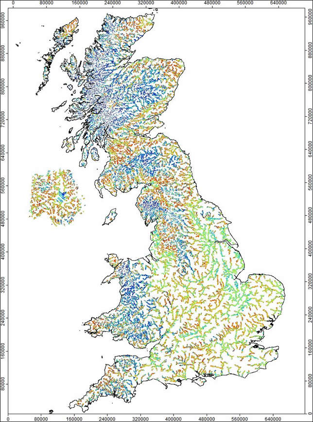

Figure
20: Possible Roman marching camp locations in Britain for the Group
65-70 hectares. The blue to light green areas are locations which do
not match the attributes well for known camps and are less likely to
have been selected. Yellow to red areas increasingly match the
attributes of the known camps and are more likely to have been
selected.


Figure
21: Possible Roman marching camp locations in Britain for the Group
50-60 hectares. The blue to light green areas are locations which do
not match the attributes well for known camps and are less likely to
have been selected. Yellow to red areas increasingly match the
attributes of the known camps and are more likely to have been
selected.
Secondly,
the south and south-east of England is a relatively dry area and
river flows are correspondingly low, and with therefore a limited
capacity to satisfy the needs of large armies. The result is that the
density or frequency of suitable rivers in southern England is low in
comparison to, say, Scotland or Wales. Consequently, the density of
strings of possible camp locations in Kent, Surrey and Sussex is far
lower than regions further west and north. This simple, some might
say even obvious, observation has implications for the account of the
Roman invasion of Britain in 43AD, which will also be explored in a
later essay.
Thirdly,
from the location of camps and roads it is apparent that the Roman
army traversed Britain either by direct march along suitable river
valleys, or placed roads and camps so that army units journeyed from
one river valley to the next. A classic example is that part of
Akeman Street that joins Cirencester with Bicester (more properly the
vexillation fortress at Alchester),
see Figure 25. Additionally, in largely unfavourable landscapes that
are inimical to marching units, by the standards defined in this
study, the Romans may have sought infrequent but suitable camp sites,
and used these as stepping-stones to advance.
Fourthly,
it might be thought when viewing Figures 20 and 21, and the
intersections of camp site locations, Roman roads, forts and towns,
that the Romans in Britain had a fundamentally sound appreciation of
the topography and hydrology of the island. It appears that this
understanding allowed the Roman military to move across, and reside
within, the landscape in a manner probably not emulated again until
the modern era. There will have been local considerations for the
placing of camps, forts and the like, but this study suggests that
there may have been an overriding understanding and plan for the
whole of Britain, possibly a plan first promulgated before the
original invasion with information supplied by traders etc. and the
earlier invasion of Julius Caesar. What is clear from the
distribution of known camps, roads, etc. is that the Romans did not
advance their campaigns into hostile territory without foreknowledge
of the allowable possibilities within the constraints imposed by the
terrain and hydrology. In emphasis, a present-day graduate of The
Royal Military
Academy Sandhurst might have a lot of knowledge and understanding in common
with a Roman army surveyor or senior officer.
Many
more generalised observations could be written but time and space
preclude, so we now turn to the amalgamation of marching camp and
hydrology data with another Roman army infrastructure, namely, Roman
roads.
The
amalgamation of marching camps, hydrology and Roman roads.
The
Roman road system known today is the result of a mixture of military
and civilian needs, Figure 22. This is especially true for England
but less so for Scotland and Wales. Indeed, it can be argued that all
Roman roads in Scotland, as few as have been found, are solely due to
the military. Self-evidently the distinction between military and
civilian use is important in the present study but, for this 'first
attempt', the two provenances have not been differentiated in the
computations discussed in the following passages.
To
put the roads in context we shall examine their initial raison d'être.
Roman army commanders planned their tribal-conquest-campaigns on
controlling the terrain, the indigenous but non-military people
(those who produced the foodstuffs) and critical navigation
pinch-points (passes, fords, navigable river intersections and the
like). Typically, they operated in the lowland areas of the tribes to
be conquered. This last point is not meant to imply that Roman units
did not advance to some form of engagement in upland areas, but that
would have been a secondary strategy followed after establishing
control in the lowlands. In general terms, the Romans conquered
tribes by firmly establishing their lines of advance, in expectation
that the tribes would engage the whole army in battle. If not, then
they controlled the productive land, starving and debilitating the
warriors, and then engaged them either en-masse or piecemeal within
the margins of the controlled area, the uplands or other
non-productive regions: i.e. advance, control and then conquer.
Support
for this concept comes from Frontinus, a Roman writer of the 1st century AD, when he supposedly quotes Julius Caesar: “I
follow the same policy toward the enemy as do many doctors when
dealing with physical ailments, namely, that of conquering the foe by
hunger rather than by steel”; a reference to the policy of controlling supply and support to the
warriors.
Necessarily,
the main Roman advance would have been by the river valleys or
broader lowland areas with rivers capable of supplying the main army.
This form of advance is exemplified by the routes taken in Scotland
(Figure 22) where most roads have been found skirting the upland and
highland regions. (As an aside: other roads within the higher ground
may have existed but have not been located yet. The same may be true
of much of Wales and parts of England, especially the south-west).

Figure
22: Roman roads of Britain, military and civilian undifferentiated.
Sources: Royal Commission on the Ancient and Historical Monuments of
Wales, Royal Commission on the Ancient and Historical Monuments of
Scotland and English Heritage. Elements of this image are ©
Crown Copyright. All rights reserved 2013.
Of
course, wherever the main Roman army advanced it built marching camps
and, because of the need for rapid and secure supply, communication
and reinforcement, it linked the camps by road. This leads to the
main supposition of this section; places where streams and rivers
with sufficient flow to satisfy the army unit's demand are
intersected by roads would have been a very favourable location to
build a marching camp. However, there are complications.
The
primary source of complication arises from the simple fact that an
army advancing into unconquered territory does not move as quickly as
one moving through an already conquered land, where the
infrastructure of roads and pre-existing camps is already in place.
This observation is further complicated by realising that the speed
of advance into hostile land is greatly determined by the size of the
army: larger equals slower. These factors are the simple consequence
of moving bodies of men and equipment from camp-to-camp during
daylight hours and, crucially, without a pre-existing road. Of
course, there were other contributing factors that created
variability in the speed of advancement, such as increased terrain
ruggedness or the aggressiveness of the opposition.
The
corollary is that the rearward areas have a faster movement rate and
it is thought reasonable that the Roman army would have adjusted the
distance between marching camps accordingly, thereby improving the
efficiency of supply, communication and reinforcement. To be clear,
if the advancing head of the army moved at 15 km/day, then that is
the distance between the initial marching camps. Meanwhile, the rear
of the army might have been capable of 25km/day, and that would be
the optimum distance between marching camps to the rear of the
advancing units. Possibly, even necessarily therefore, in the rear
areas some advance camps would be abandoned as being quite literally
out-of-step, and new ones built to enable the increased day-to-day
cadence.
Furthermore,
once the area was fully conquered then the process of re-adjustment
probably continued as the Roman army matched the camp and road
infrastructure to its marching capabilities. Probably the most common
cadence between camps would be 29km, the frequently quoted daily
marching rate of legionaries. However, 29km/day is too fast for less
agile traffic, e.g. ox-drawn wagons at c.12km/day, and indeed may not
have been the preferred peace-time marching rate of the legionary.
Therefore, set between the 29km camps would have been other camps
with a lower cadence.
Clearly,
the comments in the last paragraphs point to a complex evolution of
the camp and road infrastructure as territories transformed from
hostile to Romanized in nature; a complexity that, at this early
examination stage, makes it difficult to posit assured claims for
probable, as opposed to possible, camp locations. Regardless,
producing maps of the intersections of rivers and roads is
beneficial.
To
that end, and taking the example of Suetonius Paulinus' army during
the Boudican uprising of 60 or 61 AD of probably 10,000 'armed men',
2,500 servants, 2,500 civilians, 3,000 mules and 937 horses, maps of
river-road intersections were produced by GIS techniques from the
datasets already described.
The
figure for 'armed men' is given by Tacitus, while those of servants,
civilians and beasts are the author's. It is a total of 15,000
humans. To maintain correspondence with the statistics already
computed during this study, the known marching camp of Carstairs Main
in Scotland, a member of the Group 18 hectares, was used as a
surrogate for Suetonius' army: 11,592 soldiers, 2,898 servants, 2,898
mules and 543 horses; a total of 15,033 humans. This camp covers an
area of 16.8 hectares, and the complement of humans and beasts
described requires a minimum of 0.004255 cumecs from an adjacent
river. This is doubled to 0.00851 cumecs to produce the river flow
figure thought in this study to be the minimum a surveyor would find
acceptable.
The
GIS task is now to define a region around the possible camp that
would be used firstly to extract a suitable attribute range from the
statistical grids produced earlier (example in Figure 19), and
secondly to define the size of the possible camp ground surrounding
the river-road intersections. The former was achieved by simply
selecting only those grid cells that had 7 or more summed attributes
in the group-attribute-grid for the Group 18 hectares. The latter was
achieved by taking the half of the average side-length of the Group
18 hectare camps and summing with the mode of the distance to the
rivers that supplied an excess of water to the same group, i.e. 200
metres, giving a total of 406 metres. This is a conservative measure
as the mode of the first-river distances
from camps for Group 18 hectares is only 50metres.
Using
these parameters, 0.00851 cumecs of flow for the rivers and the
sub-selected group-attribute-grid values, in combination with the 406
range limit around river-road intersections, allows the production of
a map showing the most favourable camp locations across Britain.
Unfortunately, the scale of detail and the limits of this medium
preclude the display of a map of Britain. However, interested readers
can download higher resolution Tiffs files for all the groups
described in this essay at the top of this essay.
As
an example of the output, Figure 23 shows the river-road intersection
locations in central-southern England for camp sites suitable for
15,000 humans, i.e. Carstairs Main, as a proxy for Suetonius
Paulinus' army.

Figure
23: The most suitable Roman marching camps locations, the blue and
red patches, at river-road intersections in central-southern England
for an army of 15,000 humans (known camp Carstairs Main, Group 18
hectares). Red patches are locations with a full compliment of
attributes: blue patches one less. Roads are black. Elements of this
image are © Crown Copyright. All rights reserved 2013.

Figure
24: The most suitable Roman marching camps locations, the blue and
red patches, at river-road intersections in central-southern
England, plus, camp grounds alongside rivers, the light-green
worm-like structures. The data is derived from the statistics for an
army of 15,000 humans (known camp Carstairs Main, Group 18 hectares).
Red patches are locations with a full compliment of river-road
attributes: blue patches one less. Roads are black. Elements of this
image are © Crown Copyright. All rights reserved 2013.
The
full benefit of the methods discussed becomes more apparent when both
the river-road intersections and camp grounds alongside rivers are
displayed together (Figure 24). When viewing this image, it is
important to recall that the roads have not been differentiated
between military and civilian, that not all roads have yet been
found, and that less favourable road and river grid cells, i.e. those
with a lower attribute count, are not displayed.
This
essay is primarily designed to describe the methods employed to
produce such maps, not to describe the maps themselves, as this in
itself a huge task and requires detailed local knowledge.
Nevertheless, to demonstrate some of the information that can be
extracted from these maps we will discuss Akeman Street between the
vexillation fortresses at Cirencester and Alchester (modern
Bicester), Figure 25. This road traverses approximately WSW-ENE while
crossing the southern margin of the high Cotswolds, north of the
Thames river valley.

Figure
25: The Roman road Akeman Street between the vexillation fortresses
at Cirencester and Alchester.
Colours as for Figure 24. Elements of this image are © Crown
Copyright. All rights reserved 2013.
The
river Windrush is a major tributary of the Thames, and flows at a
rate of 0.45 cumecs at the village of Asthall during August. This is
more than sufficient for the largest Roman army that marched in
Britain. It will be remembered that the standard legionary marching
rate is 29km/day. Asthall is located 30km from Alchester and 29km
from Cirencester, that is, the journey would take exactly two days,
and this correspondence with the marching rate is possibly no
accident. Also, the Windrush at Asthall has the highest flow rate of
all the rivers between Cirencester and Alchester, except for the
Cherwell which is only 8km west of Alchester. Therefore, Asthall
appears to be perfectly located along Akeman street to satisfy the
movement of the legions. Other river-road intersections, the red and
blue patches in Figure 25, are typically 5 to 8 km apart, with one
section being 10 km long, which is a distance between water and night
stops that would suit heavy oxen-drawn carriages. A simple conclusion
might be that the road has been engineered, even fine-tuned, to match
the needs of the various types of traffic. If this is so, then
clearly not only was distance an important design factor, but also
the availability of sufficient water at the stopping places.
These
observations, based on the river-road and other camp defining
attributes, are supported by the archaeological record for Alchester.
For example, finds suggest Roman settlement occupation from the 1st to 4th centuries AD and it is postulated that one larger building may have
been a mansio (a governmental building and facilities maintained for
travellers.) A camp of 86 x 97 metres and aligned to Akeman Street
was found 1.5 km south-west from the crossing point at Asthall.
However, there is no near-by water supply. The English Heritage
website does not state what sort of camp this might have been,
however Welfare and Swan (see primary references) have it as an addendum in their work on English Roman
camps. This areal size matches that for the known marching camp at
Langwathby Moor in Cumbria which, at a density of 690
soldiers/hectare, would have held 552 soldiers, 138 servants and
mules and 25 horses, requiring 0.00021 cumecs of water. However, as
the Asthall camp is water-deficient it would seem, on the basis of
the findings in this study, that it was probably not a marching camp
for the military.
In
conclusion, this simple examination of Akeman Street and Asthall is
an example of what can be deduced from the method and maps presented
in this essay.
Further
examples will be written in the future and placed on the author's
website at www.bandaarcgeophysics.co.uk/arch_intro.html
Appendix 1: Limitations and caveats
The
work described in this essay will be improved as new data and
techniques are investigated, meanwhile, the following points outline
the limitations and caveats the author considers most important.
-
The
majority of the findings are derived from SRTM data at a grid
spacing of 90 metres. This spacing limits the resolving power of
many of the techniques. The author is hopeful of acquiring a sound
topographical dataset at a higher resolution: 50 or more preferably,
25 metres.
-
The
hydrology calculations are based on the SRTM 90 metre data and
consequently suffer from the limitation of resolution discussed in
point 1). The author hopes to acquire a sound hydrological grid in
the future.
-
The
method used to calculate the river flow statistics is based
primarily on rainfall, evapotranspiration and surface flows. It does
not involve calculations of ground water processes, for example,
aquifer discharge to rivers. Additionally, the naturalised flow
calculations are at the very extreme of what is thought possible
given the minimal flows involved; consequently, some postulated
battle sites, located alongside rivers supplying the minimum of
demand, may not be viable. Nevertheless, the present results are
surprisingly well-correlated with the limited published data from
the Centre for Ecology & Hydrology (CEH).
-
Due
to the SRTM limitations already mentioned, the width and breadth
measurements of the Roman marching camps were not used to extract
the various indices used in the study. Instead a simple, circular
buffer was placed at the known centre of the camp, the radius of
which was based on the longest known side of the camps. This is
thought to be acceptable at a 90 metre resolution, but not so if the
base grid is improved in the future to 50 or 25 metres.
-
The
SRTM 90 metre grid described above limits the resolution of all
resultant calculations and, necessarily, creates some location
'jitter' in the placement and calculation of factors related to
rivers, roads and various attributes. This 'jitter' has its most
obvious effect at the 10s of metre scale but does also effect larger
measures of scale, size and attributes resulting from calculations
based on these scales.
-
The
Roman road dataset has not been parsed to separate those built and
used by the military from
those of civilian construction and use. It could be argued that
most, if not all, roads in Scotland and Wales are military, but that
is not the case for England. These issues will be tackled in future
work.
-
Much
of the prediction of marching camp locations is based on the
selection of various statistical methods thought most applicable to
the issue at hand. Therefore, there exists a subjectivity in the
methods selected. This is unavoidable in most cases, and will
theoretically always be the case, nevertheless it is hoped to
improve the statistical methodology after the resolution and
hydrological issues have been solved (points 1 and 2).
Primary
references for marching camps:
Welfare, H and
Swan, V. 1995. Roman Camps in England. The Field Archaeology. RCHME, London.
Davies, J.L.
And Jones, R.H. 2006. Roman Camps in Wales and the Marches.
Univ. of Wales Press, Cardiff.
Jones, R.H.
2011. Roman Camps in Scotland. Society of Antiquaries of
Scotland, Edinburgh.
Jones, R.H.
2012. Roman Camps in Britain. Amberley Publishing, Stroud.
The
Royal Commission on the Ancient and Historical Monuments of Scotland(RCAHMS) http://canmore.rcahms.gov.uk/
Royal
Commission on the Ancient and Historical Monuments of Wales (RCAHMW) http://www.coflein.gov.uk/
English Heritage at http://www.pastscape.org.uk/default.aspx
Primary
references for Roman logistics:
Roth,
Jonathon. 1999. The
Logistics of the Roman Army at War (264 B.C. - A.D.235). Columbia
Studies in the Classical Tradition.
Peddie,
John. 2005. Conquest: The Roman Invasion of Britain. Sutton
Publishing.
Army
Veterinary Department, Great Britain. 1908. Animal
Management. Printed for H.M.S.O by Harrison and Sons.
Force
Development Directorate United
States Army. 2008. Water
Planning Guide
U.
S. Army engineer research and development laboratories, Fort Belvoir,
Virginia. 1965/6? Human waste studies in an occupied
civil defense shelter.
Primary
references for hydrology:
Marsh,
T. J. and Hannaford, J. (Eds). 2011. UK
Hydrometric Register. Hydrological data UK series. Centre for Ecology & Hydrology.
Gustard,
A., Bullock, A. and Dixon, J. 1992. Report
No. 108. Low flow estimation in the United Kingdom. Institute of Hydrology (NERC).
Gustard,
A., Marshall, D., and Sutcliffe, M. 1987. Report
No. 101. Low flow
estimation in Scotland. Institute of Hydrology
(NERC).
Smakhtin,
V. 2001. Low Flow Hydrology: a review. Journal of Hydrology,
240, 147–186
Primary
software:
SAGA,
System for Automated Geoscientific Analyses, http://www.saga-gis.org/en/index.html
Primary
dataset:
Shuttle
Radar Topography Mission (SRTM), Jarvis A., H.I. Reuter, A. Nelson, E. Guevara, 2006, Hole-filled seamless
SRTM data V3,
International Centre for Tropical Agriculture (CIAT), available from http://srtm.csi.cgiar.org.
Copyright:
This
essay is Copyright © Steve Kaye and protected under UK and
international law. May be used free of charge. Selling without prior written
consent prohibited. Obtain permission before redistributing. In all
cases this notice must remain intact.
Elements
within this essay, including the original marching camp data and
Roman roads, are © Crown Copyright. All rights reserved 2013.
This copyright is acknowledged for all images and text in which such
elements reside.
Acknowledgement:
I
thank Nici Lilley for bravely editing my quasi-Victorian grammar and
word-structure.